Monte Carlo

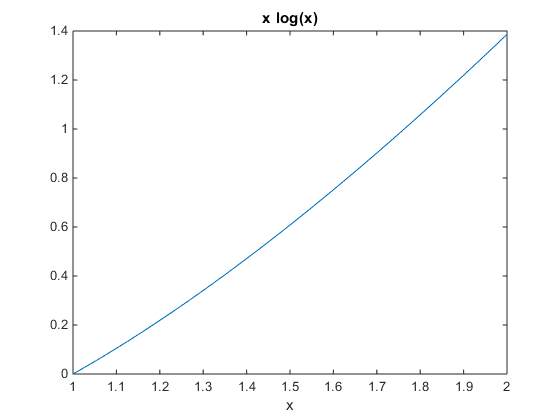
The area under the curve or has been a problem that has always been of interest to mathematicians. The advent of faster computers and processing has expanded the types of elementary functions that we can integrate, thereby enabling us to generate the graphics of complex figures in 3-dimensions. This volume problem can be thought as a solid of revolution that is obtained by rotating a plane curve around some axis. To approximate the area the under the curve we implement the Monte Carlo algorithm, Composite Trapezoidal, Simpson’s and Midpoint. With few restrictions on the integrand the Monte Carlo method can be extended to solve higher dimensional integrals though we will focus on the 2 dimensional case for the purposes of this project.

In numerical analysis the method used in approximating a definite integral is called numerical quadrature. It relies on choosing distinct nodes from the interval and then integrating the Lagrange interpolating polynomial of degree n. The Trapezoidal Rule is derived by integrating the Lagrange interpolating polynomial of degree one. Similarly, Simpson’s Rule is derived by integrating the polynomial of degree two. These algorithms are called deterministic because in their computation they evaluate a mathematical function and therefore always produce the same result. Monte Carlo integration on the other hand uses a non-deterministic approach which means that each time it is used to compute a definite integral it will produce different results. For our particular project we chose to approximate the integral using uniform random sampling.

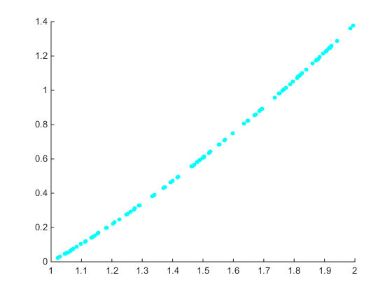
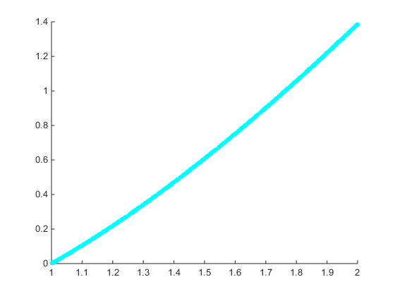
We define to be a uniform random variable in the interval . Then the point will be in and it is also a random variable that we will call . The idea behind the Monte Carlo Integration is to average samples of the function on and then multiply by the length of the interval which is . The N-th Monte Carlo Estimator is given by: .

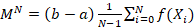Substituting in the value of and modifying the sum we obtain 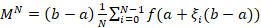. Then we proceed by taking the expectation of both sides:

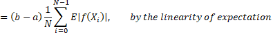
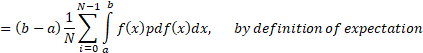
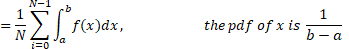
Thus, we have obtained an approximation to the integral by using the N-th Monte Carlo Estimator . The accuracy of the Monte Carlo method relies on N, the number of samples. Indeed, as the number of samples are increased the method becomes a closer approximation to the integral . This is due to the Law of Large Numbers in other words 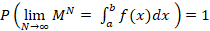guarantees that the method will converge to the exact solution for a large N.

The Monte Carlo algorithm was used to approximate and 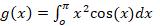with an error tolerance of and , respectively, to account for the randomness of the algorithm. The number of samples was set at 100, 1000, and 10,000.

N	function	# of trials	Integral Value	Monte Carlo	Trapezoidal	Midpoint	Simpson’s
100	f(x)	347	0.6362943611	0.6363749688	0.6363001373	0.6362832574	0.6362943612
100	g(x)	1151	-6.2831853072	-6.2834827223	-6.2837021040	-6.2821915685	-6.2831852052
1,000	f(x)	245	0.6362943611	0.6362310105	0.6362944189	0.6362942461	0.6362943611
1,000	g(x)	689	-6.2831853072	-6.2824721500	-6.2831904749	-6.2831750129	-6.2831853072
10,000	f(x)	16	0.6362943611	0.6363200205	0.6362943617	0.6362943600	0.6362943611
10,000	g(x)	3	-6.2831853072	-6.2831875750	-6.2831853589	-6.2831852039	-6.2831853072

On this particular trial, for , the Monte Carlo estimator at N=100 was able to reach the desired accuracy with relative error of .012%. When the number of iterations is increased by a factor of 10 the relative error is .009% which is a decrease of 75% from N =100. For N =10,000; the relative error is .004% which is around a 50% decrease from N = 1000. This is consistent with the law of large numbers as the error becomes smaller as the number of samples is increased. For , the relative error for N=100 is .004%, at N=1000 the relative error is .01% which is higher than expected. At 10,000 samples the error has gone down significantly to .00003%. The results indicate an interesting phenomenon, namely that as the number of samples is increased fewer trials have to be run in order to achieve the desired accuracy. This can be explained more concretely with the central limit theorem as the method has convergence then quadrupling the number of samples should decrease the error in half.

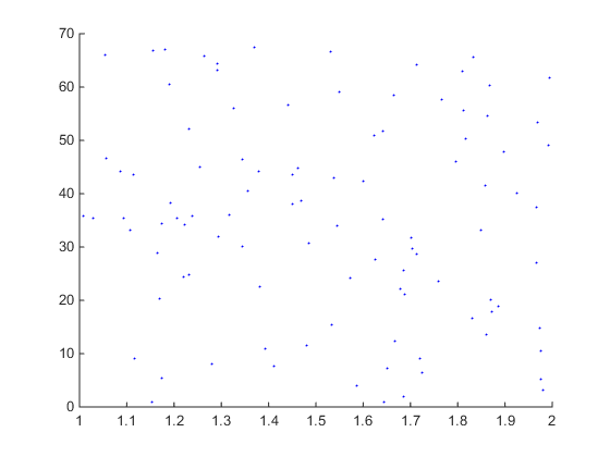
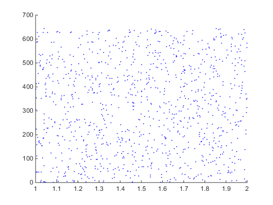
It took the Monte Carlo estimator 1151 trials to obtain an error below when integrating at N = 100, while for N = 10,000 the algorithm was able to obtain an error below in 3 trials. Similarly, the function was able to reach a tolerance of in 347 trials, at N = 100, while for N =10,000 it only took 16 trials. A major drawback in using the Monte Carlo algorithm is that the computation time becomes longer as more samples are used. This is due to the fact that we are evaluating the function at N points. To further complicate this issue is the fact that a lower error tolerance implies more trials. This is the primary reason the error tolerance was set at for the function ). On a particular run, at N=100, the algorithm took over 18,000 trials to obtain an error below and at N=10,000 it took over 700 trials.

On the other hand the deterministic algorithms perform much better since they do not rely on a random variable. Instead these algorithms divide the problem into N subintervals and carry out the method for each interval. For example, the Composite Trapezoidal method, for at N=100, was able to get an error less than in one evaluation. The Monte Carlo method took 347 tries to get an error less than . Through its divide and conquer approach the Trapezoidal method was more efficient in obtaining an approximation. The error term associated with this method is where hence by choosing large N we can minimize the error. This is consistent with the results as for N=10,000 the error is less than . The Composite Simpson’s method has an error term of where is as before, for at N = 100, the method was able to get an error less than . This is not at all surprising as the error term for the Composite Simpsons is bigger than the Trapezoidal therefore we expect to get the same accuracy the Trapezoidal method got for but for .

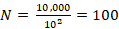The algorithms presented here are indeed the most efficient for calculating for smooth and continuous functions. They not only provide more accurate approximations but also do so in one single calculation as opposed to multiple Monte Carlo trials. To obtain the same degree of accuracy the Monte Carlo algorithm must take large N and repeat enough trials. This makes the method computationally expensive as it has to perform N function evaluations for each trial. However, the method performs well as it places few restrictions on the integrand which makes Monte Carlo an advantageous method when calculating the area under the curve of a discrete or discontinuous function. The Monte Carlo method thereby expands the types of functions we can integrate and in turn enables us to generate the graphics of complex figures in 3-dimensions.

Please send all inquiries, problems and comments to:

Email: trejo.juann@gmail.com